Residual Neural Networks as Ensembles

In a previous blog post, I had mentioned Residual Connections in the context of Google-Neural Machine Translation. I was not completely familiar with the intuition behind Residual Networks then, so heres a short post on what I gathered after reading some literature.

Residual Networks first got attention after this paper – “Deep Residual Learning for Image Recognition” by some folks from Microsoft Research. They used what they called residual connections in Convolutional Neural Networks, obtaining 1st-place results at ILSVRC 2015. However, it turns out that their notion of why the networks achieved such great performance might have been flawed.

The original authors thought that the new connections allowed training of very deep neural networks (their state-of-the-art model had 152 layers) by ‘preserving’ gradient across layers during training. This, according to them, solved the Vanishing Gradient Problem. However, the paper “Residual Networks Behave Like Ensembles of Relatively Shallow Networks” challenges this, attempting to prove that Residual NNs actually behave like ensembles of neural networks!

Lets take this step-by-step.

First, lets establish some nomenclature. In a classic neural network, suppose the output from the th layer is written as . Mathematically, you can write:

…(1)

Here, is a vectorial function that computes from . In a standard neural network, the mathematical computation performed by is same across all layers (like the ReLU). What differentiates any from other layers is the set of weights assigned to every element of towards computing elements of . These weights are of course learnt during training.

A typical layer in a Residual NN looks like this (taken from the original paper):

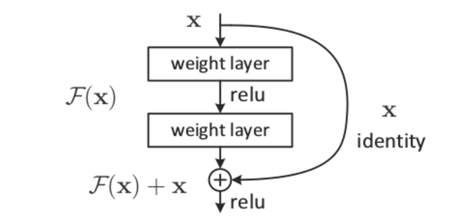
Based on our nomenclature, the expression for now becomes:

…(2)

The difference, as you must have noticed, lies in the second term on the Right-Hand-Side. This term is what they call the identity skip(or short-cut) connection. ‘Skip‘, because you are skipping the computation, and ‘identity‘ because you are not multiplying by any set of weights before addition.

These identity short-cut connections are what make residual NNs special.

‘Unravelling’ a Residual Neural Network

The reference paper‘s biggest insight lies in the way they look at equation (2) – that is, as a recursive definition. They call this unravelling the NN.

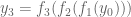
Lets consider a simple residual NN with three layers. The input can be denoted as , with the outputs from the three subsequent layers being ,  and  respectively.  is the output of the NN as a whole.

Expanding equation (2) step-by-step, we would get

…(3)

…(4)

…(5)

Equation (5) essentially defines as the sum of outputs from every single layer (including ) of the neural network.

Contrast this with what we would see if it was a standard network:

…(6)

(Ofcourse, the weights learnt would be different in each case)

Consider a situation where and the weights for are such that turns out to be a vector of very low values.

If this happens in equation (6), you see that there is very little can do. Since there is only one term on the RHS, any input basically follows one path through the NN.

But now consider equation (5). If is close to a zero vector, we still get

It looks like the input signal bypassed the second layer completely on its way to the output! In fact, if we did not have  at all, you would derive the above expression for the network. This flexibility (i.e. the ability to bypass any layer) is provided to the NN by the skip-connections.

And the ability to ‘skip’ is not just restricted to one layer per run- depending on the input and the weights at every level, any combination of them could be on/off for a given case. The name residual can be interpreted better now – residual can mean ‘unused’, which is pretty much what is in the above example! That is not the case for equation (6), since the network does not have the choice to ignore ‘s output in the single term on the RHS.

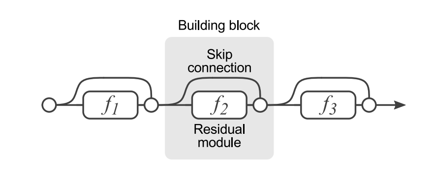
Diagrammatically, you could ‘unravel’ the network like this:

Each ‘path’ in the above figure denotes some combination of the layers working on as it makes its way to the output. Every node denotes convergence (addition) of a set of paths, before passing on the sum to the next layer.

Ideally, every output would get significant contributions from every one of those paths. But that is not usually the case, as observed by the authors of the paper.

Now lets see what happens to the figure the moment you switch off , cutting off all corresponding paths:

As you can see, even though makes no contributions, the input still makes its way through the remaining paths to generate output.

Intuitively, you can see why the authors think of this structure as an ensemble. At every single node (including the last one), there are multiple paths, any of which may or may not contribute to the overall output for a given scenario. You can say that every activates a unique set of paths in a residual NN.

And how many such paths are there? Its equivalent to the total cases resulting from every one of the layers being either on or off. Simple probability theory will tell you that its , where is the total number of layers in the NN.

Unusual properties of Residual NNs

Thinking of residual NNs as ensembles motivated the authors to conduct some experiments to test their hypothesis. Essentially, what they tried to do is see which properties of ensembles residual NNs satisfy:

1. Resilience to layer deletion: In most Neural Networks (the ones that resemble equation (2)), deleting a layer has disastrous results on the outputs – whatever the size of the overall network may be. And for good reason, as you are disrupting the one term that corresponds to the output.

But that is not the case for Residual Neural Networks. In fact, deleting 1 (or even 2 or 3) layers in large residual NNs introduces only around 6-7% of an error into the performance of the network! Moreover, deleting more and more layers actually has a pretty smooth (as in mathematically smooth) effect on the total error:

This is pretty close to how an ensemble behaves – deleting models from an ensemble does introduce error, but the increase is never drastic with respect to the number of models removed.

This can be explained easily by looking at equation (5). Even if you delete one layer from a residual NN, that still leaves terms on the RHS of the output. A bunch of them even yield the same result as they would have, with the layer in.

2. Shortening of effective paths: This is actually contradictory to what people first believed about residual NNs – that they promote deeper networks.

During training, the authors observed that the updates were not happening uniformly across all layers, as they would for normal NNs. Every training point would adjust the weights along a specific set of ‘paths’ as shown in the unravelled diagram. And most of these paths, even with 152-layer deep networks, were only 20-30 levels deep!

Even on-line, every input activated only a specific set of paths without taking significant contributions from every single layer and path in the network.

This is where the biggest revelation lies: Residual NNs work better not by increasing the effective paths, but actually reducing them! What works here is that every input has a chance to take its own unique set of paths to the output, without having to go through every single layer.

This is again similar to how ensembles are trained and run. During training, you won’t observe all smaller models in an ensemble getting significantly adjusted for every training point. On-line, there will always only be a subset of models that give a strong output for any input.

 

Thats it for now! Do read the reference paper if you feel interested, or go through the original paper to see their usage in the image processing scenario.