Weekly Review: 12/23/2017

Happy Holidays people! If you live in the Bay Area then the next week is probably your time off, so I hope you have fun and enjoy the holiday season! As for Robotics, I just finished Week 2 of Perception, and will probably kick off Week 3 in 2018. I am excited for the last ‘real’ course (Estimation & Learning), and then building my own robot as part of the ‘Capstone’ project after that :-D.

This week’s articles:

XGBoost

I recently came across XGBoost (eXtreme Gradient Boosting), an improvement over standard Gradient Boosting – thats actually a shame, considering how popular this method is in Data Science. If you are rusty on ensemble learning, take a look at this article on bagging/random Forests, and my own intro to Boosting.

XGBoost is one of the most efficient versions of Gradient Boosting, and apparently works really well on structured/tabular data. It also provides features such as sparse-awareness (being able to handle missing values), and the ability to update models with ‘continued training’. Its effectiveness for tabular data has made it very popular with Kaggle winners, with one of them quoting: “When in doubt, use xgboost”!

Take a look at the original paper to dig deeper.

Quantum Computing + Machine Learning

A lot of companies, such as Google, Microsoft, etc have recently shown interest in the domain of Quantum Computing. Rigetti happens to be a startup that aims to rival these juggernauts with its great solution to cloud-Quantum Computing (called Forest). They even have their own Python integration!

The article in question details their efforts to prototype simple clustering with quantum computing. It is still pretty crude, and is by no means a replacement to traditional systems – for now. One of the major critical points is “Applying Quantum Computing to Machine Learning will only make a black-box system more difficult to understand”. This is infact true, but the author suggests that ML could actually/maybe help us understand the behavior of Quantum Computers by modelling them!

Breaking a CAPTCHA with ML

A simple, easy-to-read, fun article on how you could break the simplest CAPTCHA algorithms with CV+Deep Learning.

Learning Indexing Structures with ML

Indexing structures are essentially data structures meant for efficient data access. For example, a B-Tree Index is used for efficient range-queries, a Hash-table is used for fast key-based access, etc. However, all of these data structures are pretty rigid in their behavior – they do not fine-tune/change their parameters based on the structure of the data.

This paper (that includes the Google legend Jeff Dean as an author) explores the possibility of using Neural Networks (infact, a hierarchy of them) as indexing structures. Basically, you would use a Neural Network to compute the function – f: data -> hash/position.

Some key takeaways from the paper:

1. Range Index models essentially ‘learn’ a cumulative distribution function.
2. The overall ‘learned index’ by this paper is a hierarchy of models (but not a tree, since two models at a certain layer can point to the same model in the next layer)
   1. As you go down the layers, the models deal with smaller and smaller subsets of the data.
3. Unlike a B-Tree, no ‘search’ involved, since each model predicts the next model for hash generation.

Tacotron 2

This post on the Google Research blog details the development of a WaveNet-like framework to generate Human Speech from text.

 

Weekly Review: 12/16/2017

Hebbian Learning in Neural Networks

One major difference between human and machine learning is the way we retain important aspects of our knowledge, as we gather more data. All throughout our life, we keep enforcing those concepts/facts which help us most in our day-to-day activities. ML algorithms are much less selective – if you train a NN to perform task A and then retrain it to perform task B, the parameters for A will be forgotten ‘uniformly’.

This paper tries to apply the Hebbian-learning principle of ‘Neurons that fire together, wire together’ to NNs. Its done as follows:

1. While training for task A, the algorithm measures the ‘importance‘ of a parameter as the gradient of the L2 norm of the output-error. In essence, this quantifies the absolute change in output for a small change in the param-value.
2. Now, while re-training for a different task, the importance values computed in the above step are used as regularization parameters. This penalizes changes to the important params for task A, even while training for task B – as a result, the NN still performs decently at task A even after being re-trained.

Distributed Tensorflow

This article gives a very good overview of distributed-computing mechanisms in TensorFlow. The main problem being tackled is the sharing of parameters/variables across different machines. Some take-aways:

1. tf.Session, by itself, is like an isolated execution engine.
2. However, multiple sessions can be made to share variables using tf.train.Servers, which are grouped together into ‘clusters’. All servers in the same cluster share variable values (this is done using namespaces).
3. With tf.device, if you have multiple devices each with their own process, you can choose which one holds the original copy of a Variable.
4. Each server is responsible for building its own Graph though – the elements of the graph can include process-specific params, as well as global ones shared across servers.

The post gives multiple small examples, as well as one cumulative piece detailed multiple feature – do take a look!

UNsupervised Image-to-Image Translation by Nvidia

Another good paper from NIPS2017. The problem addressed here is that of unsupervised image-to-image translation, also shortened as UNIT. Consider the conversion of a street-photo in sunny weather, to the same street on a rainy day.

If it was supervised, we would have pairs of photos of the same streets, in sunny & rainy weather. But such data is hard to come by, especially in the quantities needed for deep learning. So what if you just have a bunch of sunny street photos, and a set of rainy ones? (with no ‘common’ street). This is basically the problem being solved here.

Nvidia uses a VAE-GAN for this purpose, with some twists. Consider the sunny/rainy example from above:

1. The raw image is first converted to a latent vector by a Variational Autoencoder.
2. This latent vector is then given as input to the Generative part of a GAN.

The twist is that the last few layers of the VAE, and the first few layers of the GAN are shared by both sunny-to-rainy and rainy-to-sunny networks. Why so?

You can intuitively see that the VAE is converting the raw pixels into a vector encoding basic attributes of the street – irrespective of the weather. While the first few layers of the VAE deal with raw pixel data, the higher ones understand abstract street-attributes (which are weather-independent). As a result, the latter layers get shared.

The same logic is applied (but in reverse), in keeping the first few layers of the Generative network common.

Heres a video of the method to give you a taste of the results obtained. They are surprisingly good!

Fake AI porn (NSFW)

A Redditor going by the name of ‘deepfake’ uses Tensorflow-based deep learning to paste celebrity faces onto pornstar bodies in videos. While the results are not perfect, they are good enough to cause concerns over consent.

(To give you an example of the progress that has made in video manipulation, take a look at Face2Face – They use a video of some celebrity, and combine it with actions by a user on their live feed, to generate a video of the celebrity doing the same.).

Weekly Review: 12/10/2017

The Mobility Robotics course is finally done, and I just started Perception. It seems to be way more concept-heavy than any of the other courses, but I like the content from Week 1 so far! I did not like Mobility as much, since it focussed exclusively on theory, and the content assumed a fair amount of comfort with kinematics/dynamics (which I don’t have anymore). Anyway, off to the articles for this week:

AI & the Blockchain

This article gives a quick introduction to Blockchain technologies, and then delves into the relationship between Artificial Intelligence and cryptocurrencies.

It discusses the various ways in which AI could transform blockchain tech, such as: 1. Improving the energy efficiency of mining centers (like DeepMind’s algorithms do for Google), 2. Increasing scalability using Federated Learning, 3. Predicting which nodes could solve a particular block, so as to ‘free’ up the others.

Federated Learning

Coming across the mention of Federated Learning made me realise that I did not remember what it was, so I revisited the old(ish) post on Google’s Research blog.

Federated Learning works by decentralizing the training process for ML models (unlike most other technologies that mainly do inference on end-devices). This is useful in cases where communicating data continuously from devices causes bandwidth and latency issues for the user/training server.

It works like this: Every device downloads the latest version of a model from the central server. Then, as it sees more data in deployment, it trains the local model to compute small ‘focussed’ updates based on the user. All these small updates (and the not the raw data that created them) are then sent to the central server, which aggregates all the updates using the FederatedAveraging algorithm. Privacy is ensured primarily by retraining the central model only after receiving a certain number of smaller updates.

AlphaZero Chess

Sometime back, DeepMind had unveiled the AlphaGo Zero, an algorithm that learned to play Go by playing only against itself (given the basic laws of the game). They then went on to try out the MCTS-based algorithm on chess, and it seems to be working really well! The AlphaZero algorithm apparently defeated Stockfish (current computer chess champion) 28 wins to none (and a bunch of draws).

Ofcourse, the superior hardware that AlphaZero uses does make a huge difference, but the very fact that such powerful computers can be optimally used to ‘meta-learn’ is in itself a game-changer. Do read the original paper to get an idea of their method (especially the section on input/outputs Representations to the deep network)

DeepVariant

High-Throughput Sequencing (HTS) is a method used in genome sequencing. HTS produces multiple reads of an individual’s genome, which are then compared to some ‘reference’ to explore variations.

To achieve this, it is necessary to properly align the reads with the reference genome, and also account for errors in measurement. Essentially, every nucleotide position that does not match with the reference could either be a genuine variant or an error in measurement. This is determined using data from all the reads produced by the method – this problem is called the ‘Variant Calling Problem‘.

DeepVariant, an algorithm co-developed by Google Brain & Verily, converts the variant-calling problem into an image classification problem to achieve state-of-the-art results. It was unveiled at NIPS-2017, and they have open-sourced the code.

Funny Programming Jargon

This is not really an ‘article’, but more of comic relief :-). It lists out various programming terms invented by real developers, that mock the various software engineering pitfalls in a typical workplace. Do read if you appreciate programming humor!

Weekly Review: 12/03/2017

Missed a post last week due to the Thanksgiving long weekend :-). We had gone to San Francisco to see the city and try out a couple of hikes). Just FYI – strolling around SF is also as much a hike as any of the real trails at Mt Sutro – with all the uphill & downhill roads! As for Robotics, I am currently on Week 3 of the Mobility course, which is more of physics than ‘computer science’; its a welcome change of pace from all the ML/CS stuff I usually do.

Numenta – Secret to Strong AI

In this article, Numenta‘s cofounder discusses what we would need to push current AI systems towards general intelligence. He points out that many industry experts (including Jeff Bezos & Geoffrey Hinton) have opined that it would take far more than scaling up current intelligent systems, to achieve the next ‘big leap’.

Numenta’s goal as such is to take inspiration from the human brain (especially the neocortex) to design the next generation of machine intelligence. The article describes how the neocortex uses abstract ‘locations’ to understand sensory input and form mental representations. To read more of Numenta’s research, visit this page.

Transfer Learning

This article, though not presenting any ‘new findings’, is a fun-to-read introduction to Transfer Learning. It focusses on the different ways TL can be applied in the context of Neural Networks.

It provides examples of how pre-trained networks can be ‘retrained’ over new data by freezing/unfreezing certain layers during backpropagation. The blogpost also provides a bunch of useful links, such as this discussion on Stanford CS231.

Structured Deep Learning

This article motivates the need for embedding vectors in Deep Learning. One of the challenges of using SQL-ish data for deep learning, is the involvement of categorical attributes. The usual ways of dealing with such variables in ML is to use one-hot encodings, or find an integer representation for each possible value.

However, 1) one-hot encodings increase the memory footprint of a NN & 2) assigning integers to ordinal values implies a wrong meaning to neural networks, which are inherently continuous/numeric in nature. For example, Sunday=1 & Saturday=7 for a ‘week’ enum might lead the NN to believe that Sundays and Saturdays are very far apart, which is not usually true.

Hence, learning vectorial embeddings for ordinal attributes is perhaps the right way to go for most applications. While we usually know embeddings in the context of words (Word2Vec, LDA, etc), similar techniques can be used to other enum-style values as well.

Population-based Training

This blog-post by Deepmind presents a novel approach to coming up with the hyperparameters for Neural-Network training. It essentially brings in the methodology of Genetic Algorithms for designing optimal network architectures.

While standard hyperparameter-tuning methods perform some kind of random search, Population-based training (PBT) allows each candidate ‘worker’ to take inspiration from the best candidates in the current population (similar to mating in GAs) while allowing for random perturbations in parameters for exploration (a.la. GA mutations.)

 

Weekly Review: 11/18/2017

I finished the Motion Planning course from Robotics this week. It was expected, since the material was quite in line with data structures and algorithms that I have studied during my undergrad. The next one, Mobility, seems to be a notch tougher than Aerial Robotics, mainly because of the focus on calculus and physics (neither of which I have touched heavily in years).

Heres the articles this week:

Neural Networks: Software 2.0

In this article from Medium, the Director of AI at Tesla gives a fresh perspective on NNs. He refers to the set of weights in a Neural Network as a program which is learnt, as opposed to coded in by a human. This line of thought is justified by the fact that many decisions in Robotics, Search, etc. are taken by parametric ML systems. He also compares it to traditional ‘Software 1.0’, and points out the benefits of each.

Baselines in Machine Learning

In this article, a senior Research Scientist from Salesforce points out that we need to pay greater attention to baselines in Machine Learning. A baseline is any meaningful ‘benchmark’ algorithm that you would compare your algorithm against. The actual reference point would depend on your task – random/stratified systems for classification, state-of-the-art CNNs for image processing, etc. Read Neal’s answer to this Quora question for a deeper understanding.

The article ends with a couple of helpful tips, such as:

1. Use meaningful baselines, instead of using very crude code. The better your baseline, the more meaningful your results.
2. Start off with optimizing the baseline itself. Tune the weights, etc. if you have to – this gives you a good base to start your work on.

TensorFlow Lite

TensorFlow Lite is now in the Developer Preview mode. It is a light-weight platform for inference (not training) using ML models on mobile/embedded devices. Google calls it an ‘evolution of TensorFlow mobile’. While the latter is still the system you should use in production, TensorFlow lite appears to perform better on many benchmarks (Differences here). Some of the major plus-points of this new platform are smaller binaries, and support for custom ML-focussed hardware accelerators via the Android Neural Networks API.

Flatbuffers

Reading up on Tensorflow Lite also brought me to Flatbuffers, which are a ‘liter’ version of Protobufs. Flatbuffer is a data serialization library  for performance-critical applications. Flatbuffers provide the benefits of a smaller memory footprint and lesser generated code, mainly due to skipping of the parsing/unpacking step. Heres the Github repo.

Adversarial Attacks

This YCombinator article gives a nice overview of Adversarial attacks on ML models – attacks that provide ‘noisy’ data inputs to intelligent systems, in order to get a ‘wrong’ output. The author points out how Gradient descent can be used to sort-of reverse engineer spurious noise, in order to get data ‘misclassified’ by a neural network. The article also shows examples of such faulty inputs, and they are surprisingly indistinguishable from the original data!

 

Weekly Review: 11/11/2017

The Motion Planning course is going faster than I expected. I completed 2 weeks within 5 days. Thats good I guess, since it means I might get to the Capstone project before I take a vacation to India.

Heres the stuff from this week:

Graphcore and the Intelligent Processing Unit (IPU)

Graphcore aims to disrupt the world of ML-focussed computing devices. In an interesting blog post, they visualize neuron connections in different CNN architectures, and talk about how they compare to the human brain.

If you are curious about how IPUs differ from CPUs and GPUs, this NextPlatform article gives a few hints: mind you, IPUs are yet to be ‘released’, so theres no concrete information out yet. If you want to brush up on why memory is so important for neural network training (more than inference), this is a good place to start.

Overview of Different CNN architectures

This article on the CV-Tricks blog gives a high-level overview of the major CNN architectures so far: AlexNet, VGG, Inception, ResNets, etc. Its a good place to go for reference if you ever happen to forget what one of them did differently.

On that note, this blog post by Adit Deshpande goes into the ‘Brief History of Deep Learning’, marking out all the main research papers of importance.

Meta-learning and AutoML

The New York Times posted an article about AI systems that can build other AI systems, thus leading to what they call ‘Meta-learning’ (Learning how to learn/build systems that learn).

Google has been dabbling in meta-learning with a project called AutoML. AutoML basically consists of a ‘Generator’ network that comes up with various NN architectures, which are then evaluated by a ‘Scorer’ that trains them and computes their accuracy. The gradients with respect to these scores are passed back to the Generator, in order to improve the output architectures. This is their original paper, in case you want to take a look.

The AutoML team recently wrote another post about large-scale object detection using their algorithms.

Tangent

People from Google recently open-sourced their library for computing gradients of Python functions. Tangent works directly on your Python code(rather than view it as a black-box), and comes up with a derivative function to compute its gradient. This is useful in cases where you might want to debug how/why some NN architecture is not getting trained the way it’s supposed to. Here’s their Github repo.

Reconstructing films with Neural Network

This blog post talks about the use of Autoencoders and GANs to reconstruct films using NNs trained on them. They also venture into reconstructing films using NNs trained on other stylish films (like A Scanner Darkly). The results are pretty interesting.

Weekly Review: 11/04/2017

A busy week. I finished my Aerial Robotics course! The next in the Specialization is Computational Motion Planning, which I am more excited about – mainly because the curriculum goes more towards my areas of expertise. Aerial Robotics was challenging primarily because I was doing a lot of physics/calculus which I had not attempted since a long time.

Onto the articles for this week:

Colab is now public!

Google made Colaboratory, a previously-internal tool public. ‘Colab’ is a document-collaboration tool, with the added benefits of being able to run script-sized pieces of code. This is especially useful if you want to prototype small proofs-of-concept, which can then be shared with documentation and demo-able output. I had previously used it within Google to tinker with TensorFlow, and write small scripts for database queries.

Visual Guide to Evolution Strategies

The above link is a great introduction to Evolutionary Strategies such as GAs and CMA-ES. They show a visual representation of how each of these algorithms converges on the optima from the first iteration to the last on simple problems. Its pretty interesting to see how each algorithm ‘broadens’ or ‘focuses’ the domain of its candidate solutions as iterations go by.

Baidu’s Deep Voice

In a 2-part series (Part 1 & Part 2), the author discusses the architecture of Baidu’s Text-to-Speech system (Deep Voice). Take a look if you have never read about/worked on such systems and want to have a general idea of how they are trained and deployed.

Capsule Networks

Geoff Hinton and his team at Google recently discussed the idea of Capsule networks, which try and remedy the rigidity in usual CNNs – by defining groups of specialized neurons called ‘capsules’ whose contribution to higher-level neurons is decided by the similarity of output. Heres a small intro on Capsule Networks, or the original paper if you wanna delve deeper.

Nexar Challenge Results

Nexar released the results of its Deep-Learning challenge on Image segmentation – the problem of ‘boxing’ and ‘tagging’ objects in pictures with multiple entities present. This is especially useful in their own AI-dashboard apps, which need to be quite accurate to prevent possible collisions in deployment.

As further reading, you could also check out this article on the history of CNNs in Image Segmentation, another one on Region-of-Interest Pooling in CNNs, and Deformable Neural Networks. (All of these concepts are mentioned in the main Nexar article)

Weekly Review: 10/28/2017

This was a pretty busy week with a lot going on, but I finally seem to be settling into my new role!

The study for Aerial Robotics is almost over with a week to go. There hasn’t been much coding in this course, but that was to be expected since it was more about PID-Control Theory and quadrotor dynamics. I am particularly interested in the Capstone/’final’ project for this course, which would involve building an autonomous robot in Pi.

Anyway, on to the interesting tidbits from this week:

AlphaGo Zero

Google’s Deepmind recently announced a new version of their AI-based Go player, the AlphaGo Zero. What makes this one so special, is that it breaks the common notion of intelligent systems requiring a LOT of data to produce decent results. AlphaGo Zero was only provided the basic rules of Go, and it performed the rest of the learning all by playing against itself. Oh and BTW, AlphaGo Zero beats AlphaGo, the previous champion in the game. This is indeed a landmark in demonstrating the power of good-old RL.

Read this article for a basic overview, and their paper in Nature for a detailed explanation. Brushing up on Monte Carlo Tree Search would certainly help.

Word Mover’s Distance

Given an excellent embedding of words such as Word2Vec, it is not very difficult to compute the semantic distance between individual terms. However, when it comes to big blocks of text, a simple ‘average’ over term-embeddings isn’t good enough for computing their relative distances.

In such cases, the Word Mover’s Distance, inspired from Earth Mover’s Distance, provides a better solution. It figures out the semantically closest term(s) from one document to each term in another, and then the average effort required to ‘rephrase’ one text in words of another. Click on the article link for a detailed explanation.

Robots generalizing from simulations

OpenAI posted a blog article about how they trained a robot only through simulations. This means that the robot received no data from sensors during the training phase, but was able to perform basic tasks in deployment after some calibration.

During the simulations, they used dynamics randomization to alter basic traits of the environment. This data was then fed to an LSTM to understand the settings and goals. A key insight from this work is Hindsight Experience Replay. Quoting the article, “Hindsight Experience Replay (HER), allows agents to learn from a binary reward by pretending that a failure was what they wanted to do all along and learning from it accordingly. (By analogy, imagine looking for a gas station but ending up at a pizza shop. You still don’t know where to get gas, but you’ve now learned where to get pizza.)”

Concurrency in Go

If you are a Go Programmer, take a look at this old (but good) talk on concurrency patterns and constructs in the language.

Generalization Bounds in Machine Learning

The Generalization Gap for an ML system is defined as the difference between the training error and the generalization error. The Generalization Bound tries to put a bound on this value, based on probability theory. Read this article for a detailed mathematical explanation.

Weekly Review: 10/21/2017

Its been a long while since I last posted, but for good reason! I was busy shifting base from Google’s Hyderabad office to their new location in Sunnyvale. This is my first time in the USA, so there is a lot to take in and process!

Anyway, I am now working on Google’s Social-Search and Ranking team. At the same time, I am also doing Coursera’s Robotics Specialization to learn a subject I have never really touched upon. Be warned if you ever decide to give it a try: their very first course, titled Aerial Robotics, has a lot of linear math and physics involved. Since I last did all this in my freshman year of college, I am just about getting the weeks done!

Since I already have my plate full with a lot of ToDos, but I also feel bad for not posting, I found a middle ground: I will try, to the best of my ability, to post one article each weekend about all the random/new interesting articles I read over the course of the week. This is partly for my own reference later on, since I have found myself going back to my posts quite a few times to revisit a concept I wrote on. So here goes:

Eigenvectors & Eigenvalues

Anything ‘eigen’ has confused me for a while now, mainly because I never understood the intuition behind the concept. The highest-rated answer to this Math-Stackexchange question did the job: Every square matrix is a linear transformation. The corresponding eigenvectors roughly describe how the transformation orients the results (or the directions of maximum change), while the corresponding eigenvalues describe the distortion caused in those directions.

Transfer Learning

Machine Learning currently specializes in utilizing data from a certain {Task, Domain} combo (for e.g., Task: Recognize dogs in photos, Domain: Photos of dogs) to learn a function. However, when this same function/model is used on a different but related task (Recognize foxes in photos) or a different domain (Photos of dogs taken during the night), it performs poorly. This article discusses Transfer Learning, a method to apply knowledge learned in one setting on problems in different ones.

Dynamic Filters

The filters used in Convolutional Neural Network layers usually have fixed weights at a certain layer, for a given feature map. This paper from the NIPS conference discusses the idea of layers that change their filter weights depending on the input. The intuition is this: Even though a filter is trained to look for a specialized feature within a given image, the orientation/shape/size of the feature might change with the image itself. This is especially true while analysing data such as moving objects within videos. A dynamic filter will then be able to adapt to the incoming data, and efficiently recognise the intended features inspite of distortions.

 

An introduction to Bayesian Belief Networks

A Bayesian Belief Network (BBN), or simply Bayesian Network, is a statistical model used to describe the conditional dependencies between different random variables.

BBNs are chiefly used in areas like computational biology and medicine for risk analysis and decision support (basically, to understand what caused a certain problem, or the probabilities of different effects given an action).

Structure of a Bayesian Network

A typical BBN looks something like this:

The shown example, ‘Burglary-Alarm‘ is one of the most quoted ones in texts on Bayesian theory. Lets look at the structural characteristics one by one. We will delve into the numbers/tables later.

Directed Acyclic Graph (DAG)

We obviously have one node per random variable.

Directed: The connections/edges denote cause->effect relationships between pairs of nodes. For example Burglary->Alarm in the above network indicates that the occurrence of a burglary directly affects the probability of the Alarm going off (and not the other way round). Here, Burglary is the parent, while Alarm is the child node.

Acyclic: There cannot be a cycle in a BBN. In simple English, a variable cannot depend on its own value – directly, or indirectly. If this was allowed, it would lead to a sort of infinite recursion which we are not prepared to deal with. However, if you do realize that an event happening affects its probability later on, then you could express the two occurrences as separate nodes in the BBN (or use a Dynamic BBN).

Parents of a Node

One of the biggest considerations while building a BBN is to decide which parents to assign to a particular node. Intuitively, they should be those variables which most directly affect the value of the current node.

Formally, this can be stated as follows: “The parents of a variable () are the minimal set of ancestors of , such that all other ancestors of are conditionally independent of given “.

Lets take this step by step. First off, there has to be some sort of a cause-effect relationship between and for to be one of the ancestors of . In the shown example, the ancestors of Mary Calls are Burglary, Earthquake and Alarm.

Now consider the two ancestors Alarm and Earthquake. The only way an Earthquake would affect Mary Calls, is if an Earthquake causes Alarm to go off, leading to Mary Calls. Suppose someone told you that Alarm has in fact gone off. In this case, it does not matter what lead to the Alarm ringing – since Mary will react to it based on the stimulus of the Alarm itself. In other words, Earthquake and Mary Calls become conditionally independent if you know the exact value of Alarm.

Mathematically speaking, .

Thus, are those ancestors which do not become conditionally independent of given the value of some other ancestor. If they do, then the resultant connection would actually be redundant.

Disconnected Nodes are Conditionally Independent

Based on the directed connections in a BBN, if there is no way to go from a variable to (or vice versa), then and are conditionally independent. In the example BBN, pairs of variables that are conditionally independent are {Mary Calls, John Calls} and {Burglary, Earthquake}.

It is important to remember that ‘conditionally independent’ does not mean ‘totally independent’. Consider {Mary Calls, John Calls}. Given the value of Alarm (that is, whether the Alarm went off or not), Mary and John each have their own independent probabilities of calling. However, if you did not know about any of the other nodes, but just that John did call, then your expectation of Mary calling would correspondingly increase.

Mathematics behind Bayesian Networks

BBNs provide a mathematically correct way of assessing the effects of different events (or nodes, in this context) on each other. And these assessments can be made in either direction – not only can you compute the most likely effects given the values of certain causes, but also determine the most likely causes of observed events.

The numerical data provided with the BBN (by an expert or some statistical study) that allows us to do this is:

1. The prior probabilities of variables with no parents (Earthquake and Burglary in our example).
2. The conditional probabilities of any other node given every value-combination of its parent(s). For example, the table next to Alarm defines the probability that the Alarm will go off given the whether an Earthquake and/or Burglary have occurred.

In case of continuous variables, we would need a conditional probability distribution.

The biggest use of Bayesian Networks is in computing revised probabilities. A revised probability defines the probability of a node given the values of one or more other nodes as a fact. Lets take an example from the Burglary-Alarm BBN.

Suppose we want to calculate the probability that an earthquake occurred, given that the alarm went off, but there was no burglary. Essentially, we want . Simplifying the nomenclature a bit, .

Here, you can say that the Alarm going off () is evidence, the knowledge that the Burglary did not happen () is context and the Earthquake occurring () is the hypothesis. Traditionally, if you knew nothing else, , from the diagram. However, with the context and evidence in mind, this probability gets changed/revised. Hence, its called ‘computing revised probabilities’.

A version of Bayes Theorem states that

…(1)

where is the hypothesis,  is the evidence, and  is the context. The numerator on the RHS denotes that probability that  &  both occur given , which is a subset of the probability that atleast occurs given , irrespective of .

Using (1), we get

…(2)

Since and are independent phenomena without knowledge of ,

…(3)

From the table for ,

…(4)

Finally, using the Total Probability Theorem,

…(5)

Which is nothing but average of & , weighted on  &  respectively.

Substituting values in (5),

…(6)

From (2), (3), (4), & (6), we get

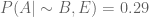
As you can see, the probability of the Earthquake actually increases if you know that the Alarm went off but a Burglary was not the cause of it. This should make sense intuitively as well. Which brings us to the final part –

The ‘Explain Away’ Effect

The Explain Away effect, commonly associated with BBNs, is a result of computing revised probabilities. It refers to the phenomenon where knowing that one cause has occurred, reduces (but does not eliminate) the probability that the other cause(s) took place.

Suppose instead of knowing that there has been no burglary like in our example, you infact did know that one has taken place. It also led to the Alarm going off. With this information in mind, your tendency to check out the ‘earthquake’ hypothesis reduces drastically. In other words, the burglary has explained away the alarm.

It is important to note that the probability for other causes just gets reduced, but does NOT go down to zero. In a stroke of bad luck, it could have happened that both a burglary and an earthquake happened, and any one of the two stimuli could have led to the alarm ringing. To what extent you can ‘explain away’ an evidence depends on the conditional probability distributions.