The basics of Likelihood

Anyone who has done some course in statistics or data science, must have come across the term ‘likelihood’. In non-technical language, likelihood is synonymous with probability. But ask any mathematician, and their interpretation of the two concepts is significantly different. I went digging into likelihood for a bit this week, so thought of putting down the basics of what I revisited.

Whenever we talk about understanding data, we talk about models. In statistics, a model is usually some sort of parameterized function – like a probability density function (pdf) or a regression model. But the effectiveness of the model’s outputs will only be as good as its fit to the data. If the characteristics of the data are very different from the assumed model, the bias turns out to be pretty high. So from a probability perspective, how do we quantify this fit?

Defining the Likelihood Function

The two entities of interest are – the data , and the parameters . Now consider a function , that returns a number proportional to the degree of ‘fit’ between the two – essentially quantifying their relationship with each other.

There are two practical ways you could deal with this function. If you kept constant and varied the data being analyzed, you would be getting a function whose only argument is the data. The output would basically be a measure of how well your input data satisfies the assumptions made by the model.

But in real life, you rarely know your model with certainty. What you do have, is a bunch of observed data. So shouldn’t we also think of the other way round? Suppose you kept constant, but tried varying instead. Now, what you have got is a function , that computes how well different sets of parameters describe your data (which you have for real).

Mind you, in both cases, the underlying mathematical definition is the same. The input ‘variable’ is what has changed. This is how probability and likelihood are related. The function is what we call the probability function (or pdf for the continuous case), and is called the likelihood function. While assumes you know your model and tries to analyze data according to it, keeps the data in perspective while figuring out how well different sets of parameters describe it.

The above definition might make you think that the likelihood is nothing but a rewording of probability. But keeping the data constant, and varying the parameters has huge consequences on the way you interpret the resultant function.

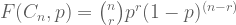
Lets take a simple example. Consider you have a set  of different coin tosses, where out of them were , while the others were . Lets say that the coin used for tossing was biased, and the probability of a coming up on it is . In this case,

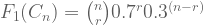
Now suppose you made coin yourself, so you know . In that case,

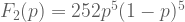
On the other hand, lets say you don’t know much about the coin, but you do have a bunch of toss-outcomes from it. You made 10 different tosses, out which 5 were . From this data, you want to measure how likely it is that your guess of is correct. Then,

There is a very, very important distinction between probability and likelihood functions – the value of the probability function sums (or integrates, for continuous data) to 1 over all possible values of the input data. However, the value of the likelihood function does not integrate to 1 over all possible combinations of the parameters.

The above statement leads to the second important thing to note: DO NOT interpret the value of a likelihood function, as the probability of the model parameters. If your probability function gave the value of 0.7 (say) for a discrete data point, you could be pretty sure that there would be no other option as likely as it. This is because, the sum of the probabilities of all other point would be equal to 0.3. However, if you got 0.99 as the output of your likelihood function, it wouldn’t necessarily mean that the parameters you gave in are the most likely ones. Some other set of parameters might give 0.999, 0.9999 or something higher.

The only thing you can be sure of, is this: If 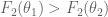, then it is more likely that denote the parameters of the underlying model.

Log Likelihoods for Maximum Likelihood Estimation

The likelihood function is usually denoted as (likelihood of the parameters given the data point ), so we will stick with it from now on. The most common use of likelihood, is to figure out that set of parameters which yields the highest value for it (and thus describes your dataset the best). This method is called Maximum Likelihood Estimation. You maximize the value of the likelihood function in a bid to find the optimal parameters for your model. This trick is applied in many areas of data science, such as logistic regression.

Maximum Likelihood Estimation usually involves computing the partial derivative of the likelihood function with respect to the parameters. We generally deal with the log-likelihood (basically the logarithm of the likelihood function) rather than likelihood itself. Since log is a monotonically increasing function, the optimum value of the likelihood function can be calculated using derivatives of log-likelihood as well. The reason we use logarithms, is to make the process of dealing with derivatives easy. Consider the coin-toss example I gave above:

Your Likelihood function for the probability of , given the and , was:

Computing log, we get

To maximise, we will compute the partial derivative with respect to , and equate to zero.

Using we get,

Solving, we get the intuitive result:

In most cases, when you compute likelihood, you would be dealing with a bunch of independent data points , rather than a single one. The likelihood of with respect to the data-set then gets defined as follows:

Using log, the overall likelihood becomes: